
How random is Java’s HashMap, really?
We treat HashMap hashing as if it’s completely random, but is it? What happens if we compare Java’s actual bucket distribution to the theoretical Poisson model?
The setup
Using Java’s Random.nextInt(), I generated 100,000 random 32-bit integer keys and inserted them into a custom HashMap implementation. The map uses chaining for collisions, a 0.75 load factor for resizing, and power-of-2 table sizes — the same fundamentals as java.util.HashMap.
int n = 100_000;
MyHashMap<Integer, Integer> map = new MyHashMap<>();
Random rand = new Random(12345); // seed for reproducibility

for (int i = 0; i < n; i++) {
    int key = rand.nextInt(); // random 32-bit key
    map.put(key, 1);
}
After insertion, I exported the size of every bucket to a CSV file and analyzed the distribution in Python.
Why Poisson?
If a hash function distributes keys uniformly at random across m buckets, then each bucket receives keys independently with probability 1/m. With n keys total, the number of keys landing in any single bucket follows a Binomial(n, 1/m) distribution. When n is large and 1/m is small — which is exactly our case — the Binomial converges to a Poisson distribution with parameter α = n/m (the average keys per bucket).
So if hashing is truly random, bucket sizes should follow:
The results
With 100,000 random keys spread across 262,144 buckets, the empirical average comes out to α ≈ 0.381.
| Statistic | Value |
|---|---|
| Buckets | 262,144 |
| Keys | 100,000 |
| Mean bucket size (α) | 0.381 |
| Variance | 0.382 |
| Max bucket size | 5 |
The mean and variance being nearly equal is already a good sign — for a Poisson distribution, the mean and variance are both equal to α.
Empirical vs. Poisson PMF
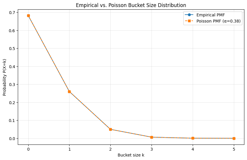
The probability mass function tells us what fraction of buckets have exactly k keys in them. Here’s the empirical PMF alongside the Poisson prediction:
| Bucket size (k) | Empirical P(X=k) | Poisson P(X=k) |
|---|---|---|
| 0 | 0.6831 | 0.6829 |
| 1 | 0.2600 | 0.2605 |
| 2 | 0.0498 | 0.0497 |
| 3 | 0.0064 | 0.0063 |
| 4 | 0.0006 | 0.0006 |
| 5 | 0.00004 | 0.00005 |
When you overlay the two distributions, they track each other closely. The shapes match — the empirical data follows the same rapid exponential decay as the Poisson model.
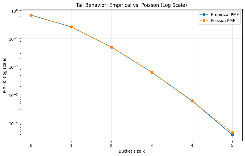
On a log scale, the tail behavior is even more telling. Both curves fall off at the same rate, confirming the match extends beyond just the peak of the distribution.
Max bucket size
There’s a well-known result for the maximum of m independent Poisson random variables:
For 262,144 buckets, this predicts a max bucket size of 4.94. The empirical max was 5 — nearly a perfect match.
What this means
The bucket size distribution from a real hashmap simulation is statistically indistinguishable from what you’d expect under perfectly random hashing. This validates the theoretical assumption behind HashMap’s O(1) average-case performance: the hash function spreads keys uniformly enough that collisions follow a predictable, well-behaved distribution.
The Poisson model isn’t just a textbook abstraction — it accurately describes what actually happens inside a HashMap.
I’ve been practicing #LeetCode and wanted to dig deeper on hashmaps — how random are hash functions really, and how does that lead to O(1) lookups? I ran a simulation and compared the results to the Poisson distribution. Check out my first blog post: https://jfischer.dev/blog/how-random-is-javas-hashmap-really/